Creator: Chung-En Johnny Yu
Content update: 2025/10/04
Source:
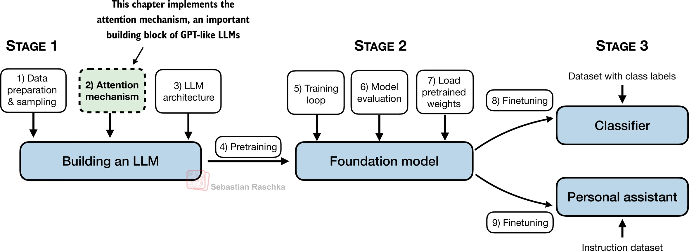
Build a Large Language Model From Scratch by Sebastian Raschka - Ch3
Hands-on practice this notebook on your Google Colab:
Now, run the code and practice it!
Additional resources (not included here):
Attention as Soft Dictionary Lookup by Yuan Meng
Understanding and Coding Self-Attention, Multi-Head Attention, Causal-Attention, and Cross-Attention in LLMs by Sebastian Raschka
Transformers Laid Out by Pramod
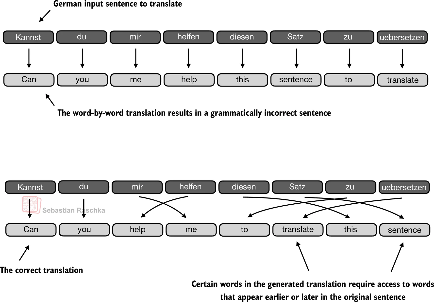
Modeling long sequences problem
Translating a text word by word isn’t feasible due to the differences in grammatical structures between the source and target languages.
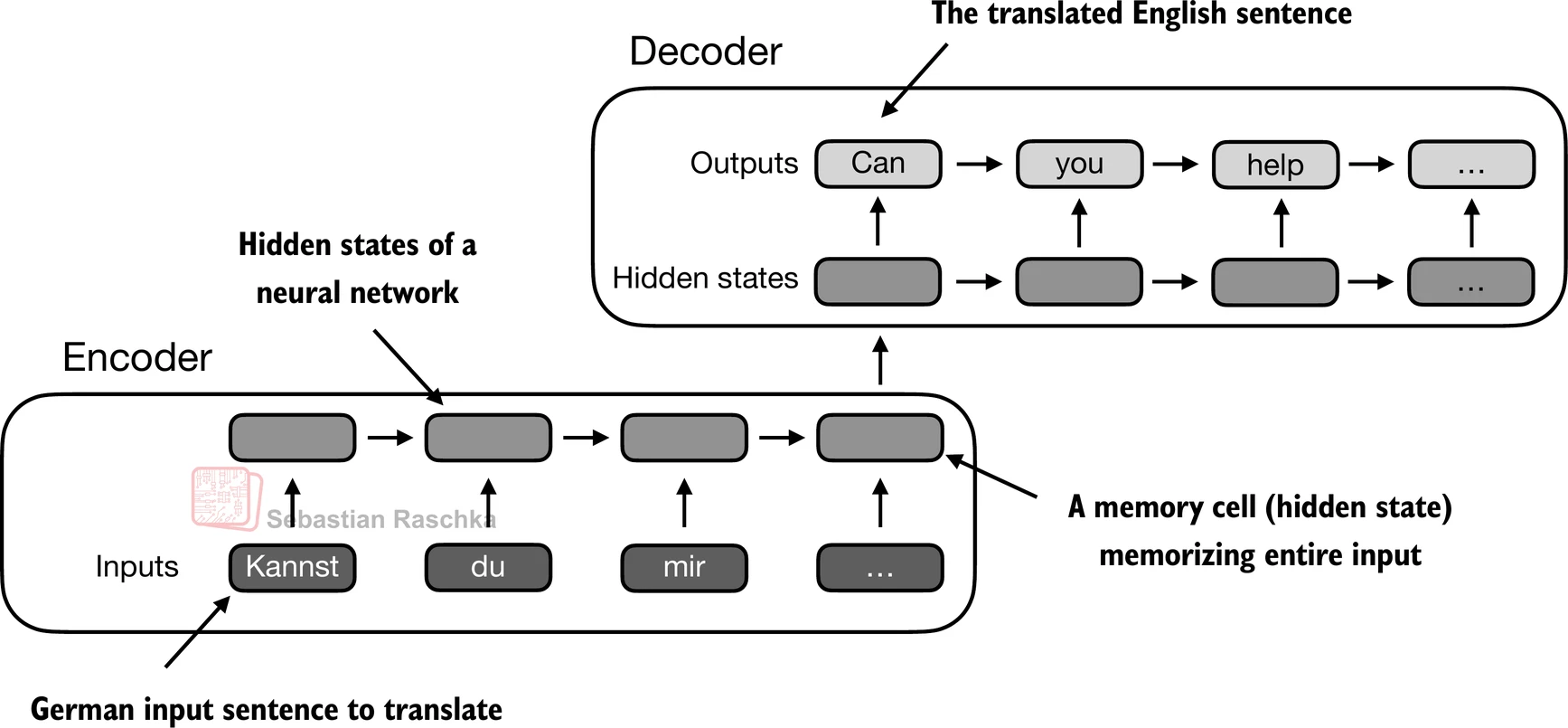
Recurrent Neural Networks (RNNs)
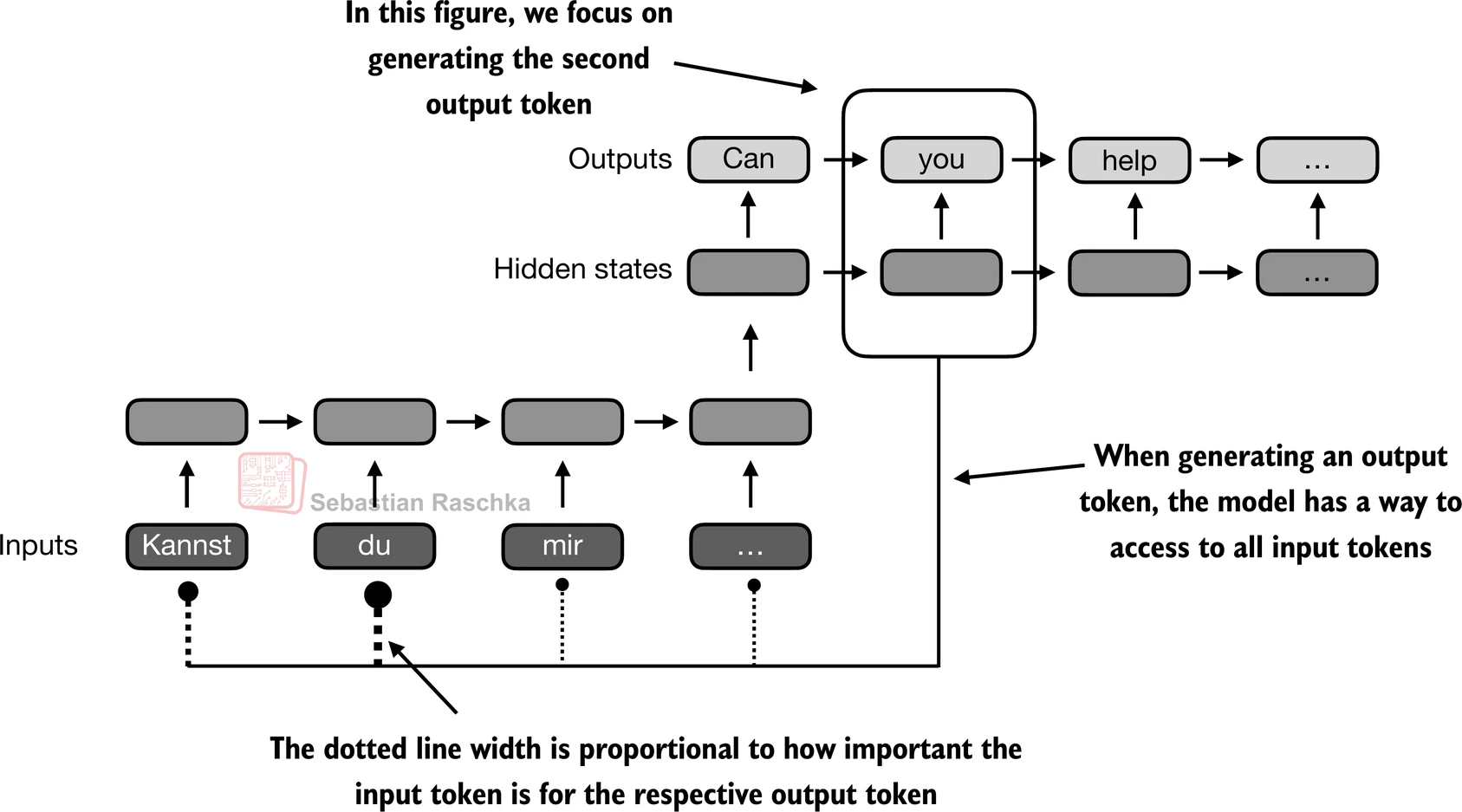
Prior to the introduction of transformer models, encoder-decoder RNNs were commonly used for machine translation tasks.
In this setup, the encoder processes a sequence of tokens from the source language, using a hidden state—a kind of intermediate layer within the neural network—to generate a condensed representation of the entire input sequence.
Problem: Can’t handle long context.
It can’t directly access earlier hidden states from the encoder during the decoding phase. Consequently, it relies solely on the current hidden state, which encapsulates all relevant information. This can lead to a loss of context, especially in complex sentences where dependencies might span long distances.
Capturing data dependencies with attention
Through an attention mechanism, the text-generating decoder segment of the network is capable of selectively accessing all input tokens, implying that certain input tokens hold more significance than others in the generation of a specific output token.
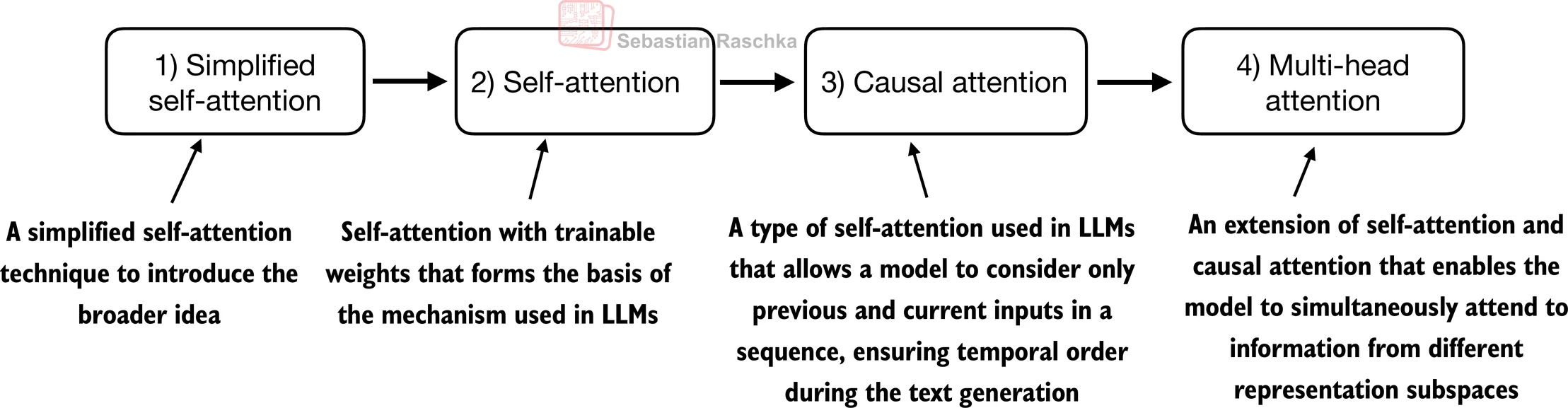
Self-attention (More in the next section)
Self-attention in transformers is a technique designed to enhance input representations by enabling each position in a sequence to engage with and determine the relevance of every other position within the same sequence.
Self-attention without trainable weights
Simple illustration
This section:
Explain a very simplified variant of self-attention, which does not contain any trainable weights.
Purely for illustration purposes and NOT the attention mechanism that is used in transformers.
Problem setup in math for the following figure:
Suppose we are given an input sequence to :
The input is a text (for example, a sentence like “Your journey starts with one step”) that has already been converted into token embeddings.
For instance, is a d-dimensional vector representing the word “Your”, and so forth.
Goal:
Compute context vectors for each input sequence element in to (where and have the same dimension).
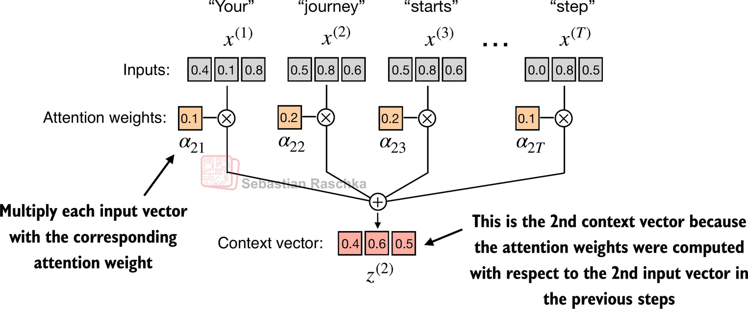
A context vector is a weighted sum over the inputs to .
The context vector is “context”-specific to a certain input.
Instead of as a placeholder for an arbitrary input token, let’s consider the second input, .
And to continue with a concrete example, instead of the placeholder , we consider the second output context vector, .
The second context vector, , is a weighted sum over all inputs to weighted with respect to the second input element, .
The attention weights are the weights that determine how much each of the input elements contributes to the weighted sum when computing .
In short, think of as a modified version of that also incorporates information about all other input elements that are relevant to a given task at hand.
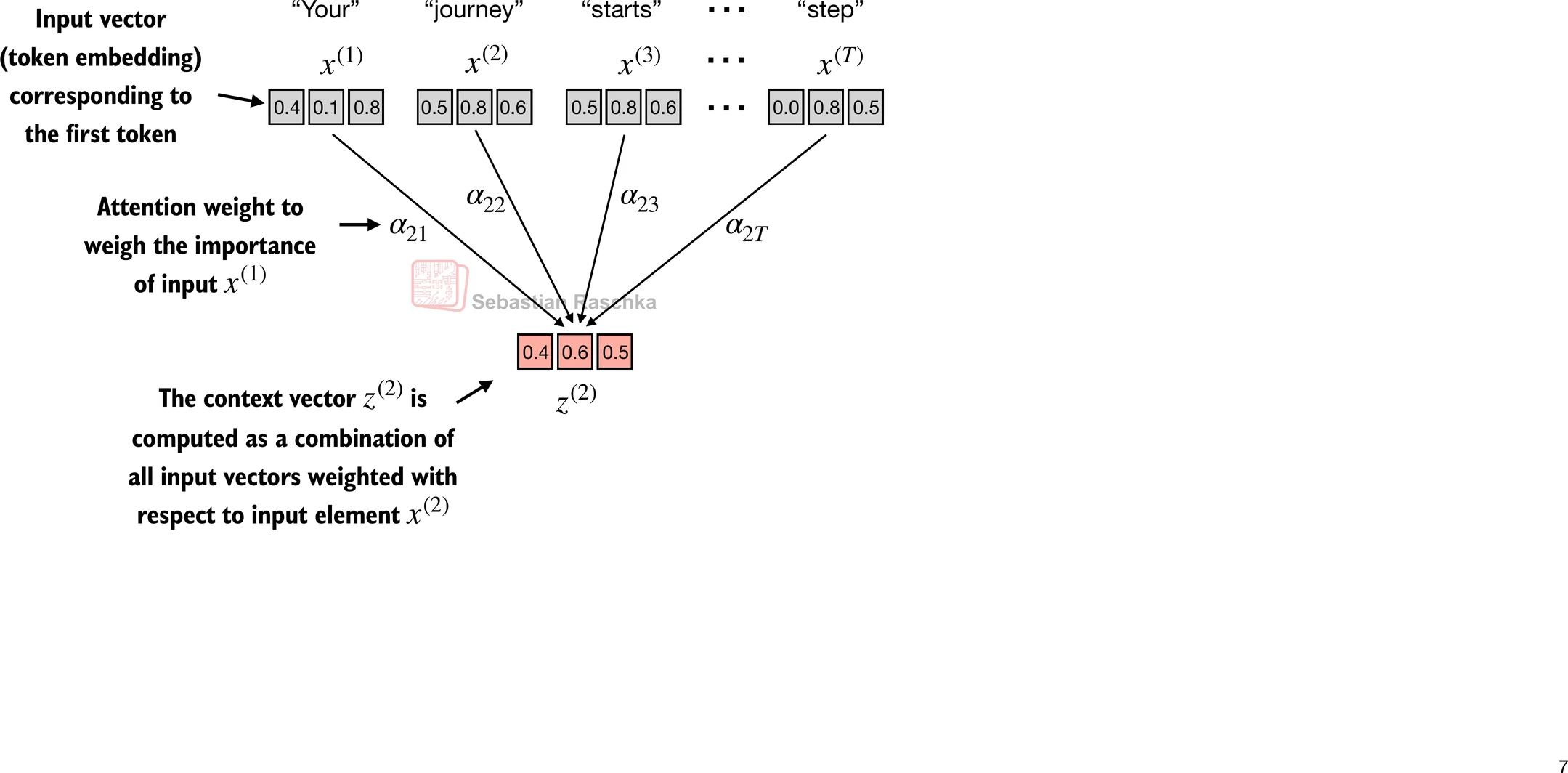
(Please note that the numbers in this figure are truncated to one digit after the decimal point to reduce visual clutter; similarly, other figures may also contain truncated values)
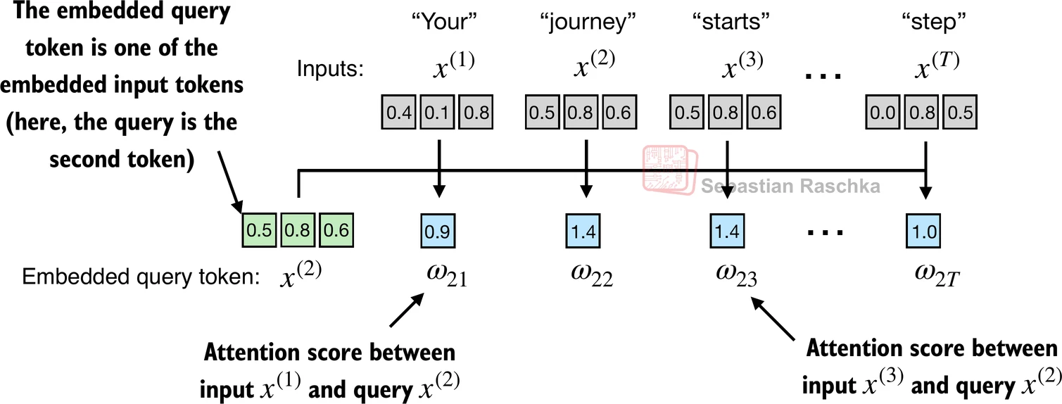
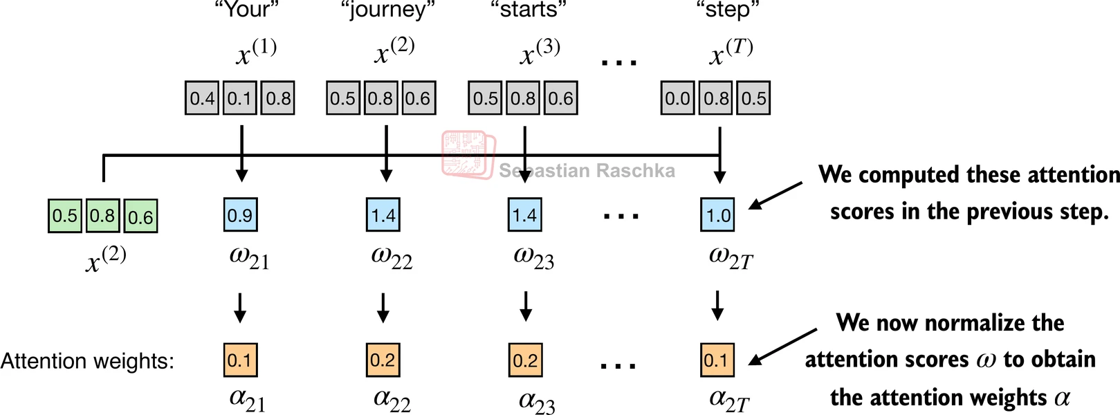
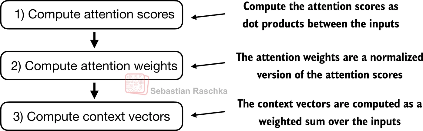
Step 1: Compute unnormalized attention scores ()
By convention, the unnormalized attention weights are referred to as “attention scores” () whereas the normalized attention scores, which sum to 1, are referred to as “attention weights” ().
Suppose we use the second input token as the query, that is, , we compute the unnormalized attention scores via dot products:
...
The subscript “21” in means that input sequence element 2 was used as a query against input sequence element 1.
from importlib.metadata import version

print("torch version:", version("torch"))
torch version: 2.8.0+cu126
import torch

inputs = torch.tensor(
  [[0.43, 0.15, 0.89], # Your     (x^1)
   [0.55, 0.87, 0.66], # journey  (x^2)
   [0.57, 0.85, 0.64], # starts   (x^3)
   [0.22, 0.58, 0.33], # with     (x^4)
   [0.77, 0.25, 0.10], # one      (x^5)
   [0.05, 0.80, 0.55]] # step     (x^6)
)
The figure depicts the initial step in this process, which involves calculating the attention scores ω between and all other input elements through a dot product operation.
query = inputs[1]  # 2nd input token is the query

attn_scores_2 = torch.empty(inputs.shape[0])
for i, x_i in enumerate(inputs):
    attn_scores_2[i] = torch.dot(x_i, query) # dot product (transpose not necessary here since they are 1-dim vectors)

print(attn_scores_2)
tensor([0.9544, 1.4950, 1.4754, 0.8434, 0.7070, 1.0865])
Step 2: Normalize the unnormalized attention scores (“omegas”, ) to get the attention weights ().
Here is a simple way to normalize the unnormalized attention scores to sum up to 1 (a convention, useful for interpretation, and important for training stability).
attn_weights_2_tmp = attn_scores_2 / attn_scores_2.sum()

print("Attention weights:", attn_weights_2_tmp)
print("Sum:", attn_weights_2_tmp.sum()) # sanity check
Attention weights: tensor([0.1455, 0.2278, 0.2249, 0.1285, 0.1077, 0.1656])
Sum: tensor(1.0000)
However, in practice, using the softmax function for normalization, which is better at handling extreme values and has more desirable gradient properties during training, is common and recommended.
attn_weights_2 = torch.softmax(attn_scores_2, dim=0)

print("Attention weights:", attn_weights_2)
print("Sum:", attn_weights_2.sum())
Attention weights: tensor([0.1385, 0.2379, 0.2333, 0.1240, 0.1082, 0.1581])
Sum: tensor(1.)
Step 3: Compute the context vector by multiplying the embedded input tokens, with the attention weights and sum the resulting vectors.
query = inputs[1] # 2nd input token is the query

context_vec_2 = torch.zeros(query.shape)
for i,x_i in enumerate(inputs):
    context_vec_2 += attn_weights_2[i]*x_i

print(context_vec_2)
tensor([0.4419, 0.6515, 0.5683])
Attention weights for ALL input tokens
Now, we are generalizing this computation to compute all attention weights and context vectors.
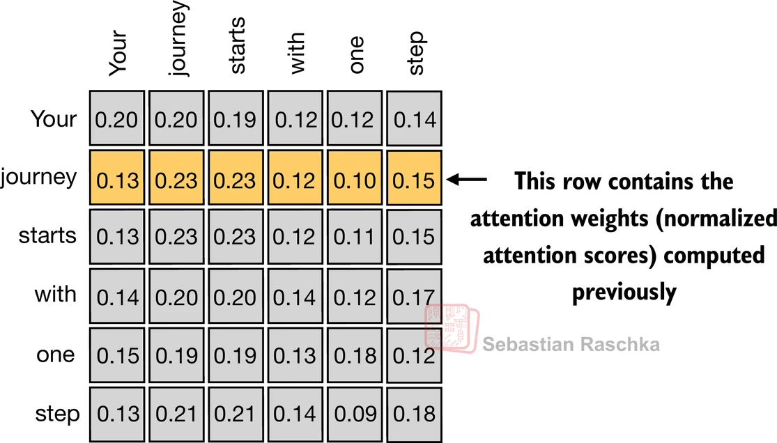
Apply previous step 1 to all pairwise elements to compute the unnormalized attention score matrix.
attn_scores = inputs @ inputs.T
print(attn_scores)
tensor([[0.9995, 0.9544, 0.9422, 0.4753, 0.4576, 0.6310],
[0.9544, 1.4950, 1.4754, 0.8434, 0.7070, 1.0865],
[0.9422, 1.4754, 1.4570, 0.8296, 0.7154, 1.0605],
[0.4753, 0.8434, 0.8296, 0.4937, 0.3474, 0.6565],
[0.4576, 0.7070, 0.7154, 0.3474, 0.6654, 0.2935],
[0.6310, 1.0865, 1.0605, 0.6565, 0.2935, 0.9450]])
Similar to step 2 previously, we normalize each row so that the values in each row sum to 1.
attn_weights = torch.softmax(attn_scores, dim=-1)
print(attn_weights)
tensor([[0.2098, 0.2006, 0.1981, 0.1242, 0.1220, 0.1452],
[0.1385, 0.2379, 0.2333, 0.1240, 0.1082, 0.1581],
[0.1390, 0.2369, 0.2326, 0.1242, 0.1108, 0.1565],
[0.1435, 0.2074, 0.2046, 0.1462, 0.1263, 0.1720],
[0.1526, 0.1958, 0.1975, 0.1367, 0.1879, 0.1295],
[0.1385, 0.2184, 0.2128, 0.1420, 0.0988, 0.1896]])
Quick verification that the values in each row indeed sum to 1.
row_2_sum = sum([0.1385, 0.2379, 0.2333, 0.1240, 0.1082, 0.1581])
print("Row 2 sum:", row_2_sum)

print("All row sums:", attn_weights.sum(dim=-1))
Row 2 sum: 1.0
All row sums: tensor([1.0000, 1.0000, 1.0000, 1.0000, 1.0000, 1.0000])
Apply previous step 3 to compute all context vectors.
all_context_vecs = attn_weights @ inputs
print(all_context_vecs)
tensor([[0.4421, 0.5931, 0.5790],
[0.4419, 0.6515, 0.5683],
[0.4431, 0.6496, 0.5671],
[0.4304, 0.6298, 0.5510],
[0.4671, 0.5910, 0.5266],
[0.4177, 0.6503, 0.5645]])
As a sanity check, the previously computed context vector can be found in the 2nd row in above.
print("Previous 2nd context vector:", context_vec_2)Previous 2nd context vector: tensor([0.4419, 0.6515, 0.5683])
Self-attention with trainable weights
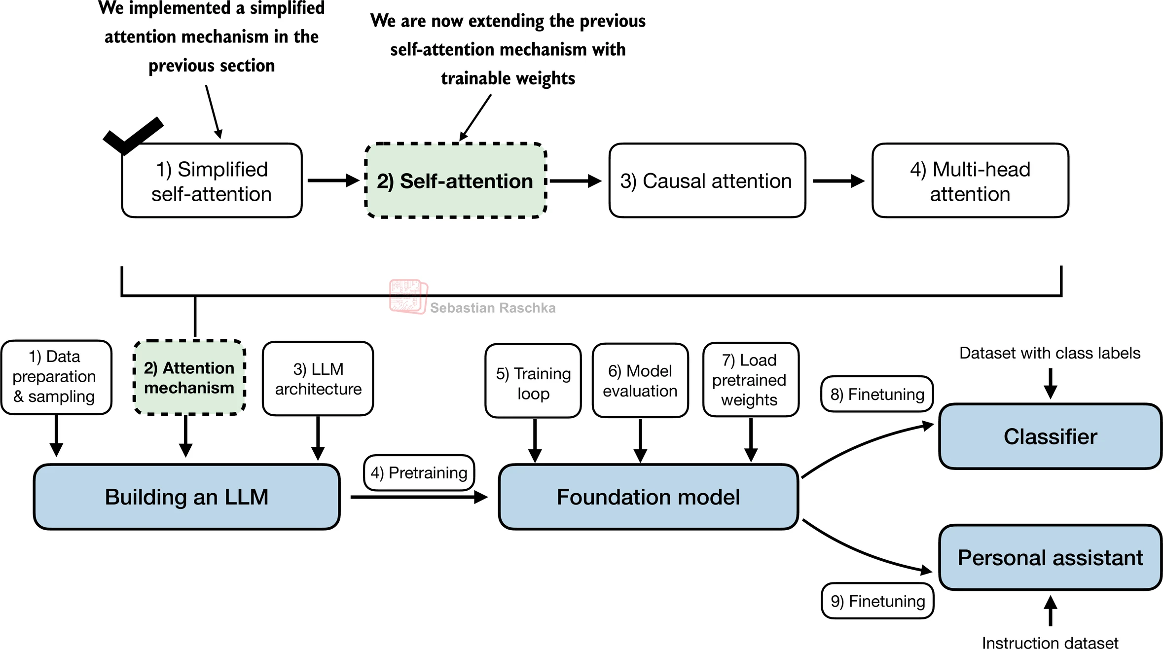
Step by step
This self-attention mechanism is also called “scaled dot-product attention”.
The most notable difference is the introduction of weight matrices that are updated during model training.
These trainable weight matrices are crucial so that the model (specifically, the attention module inside the model) can learn to produce “good” context vectors.
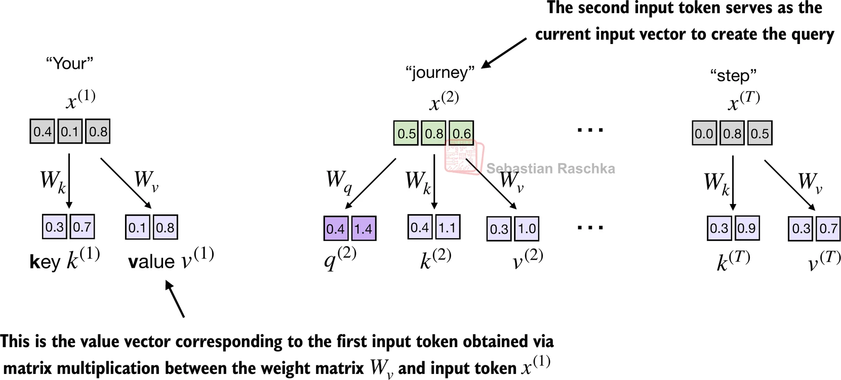
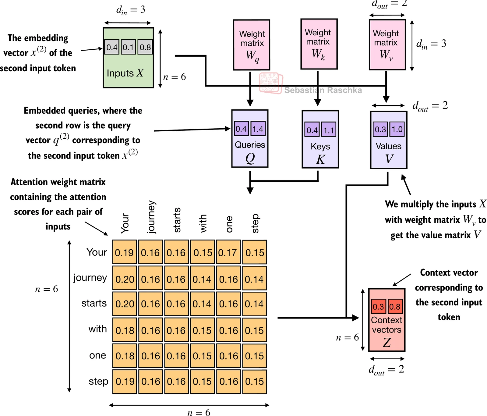
We will start by introducing the three training weight matrices , , and .
These three matrices are used to project the embedded input tokens, x^{(i)} , into query, key, and value vectors via matrix multiplication:
Query vector:
Key vector:
Value vector:
The embedding dimensions of the input and the query vector can be the same or different, depending on the model’s design and specific implementation
In GPT models, the input and output dimensions are usually the same, but for illustration purposes, to better follow the computation, we choose different input and output dimensions.
x_2 = inputs[1] # second input element
d_in = inputs.shape[1] # the input embedding size, d=3
d_out = 2 # the output embedding size, d=2
Step 1, we initialize the three weight matrices.
(Note that we are setting requires_grad=False to reduce clutter in the outputs for illustration purposes, but if we were to use the weight matrices for model training, we would set requires_grad=True to update these matrices during model training.)
torch.manual_seed(123)

W_query = torch.nn.Parameter(torch.rand(d_in, d_out), requires_grad=False)
W_key   = torch.nn.Parameter(torch.rand(d_in, d_out), requires_grad=False)
W_value = torch.nn.Parameter(torch.rand(d_in, d_out), requires_grad=False)
Next we compute the query, key, and value vectors.
query_2 = x_2 @ W_query # _2 because it's with respect to the 2nd input element
key_2 = x_2 @ W_key
value_2 = x_2 @ W_value

print(query_2)
tensor([0.4306, 1.4551])
As we can see below, we successfully projected the 6 input tokens from a 3D onto a 2D embedding space.
keys = inputs @ W_key
values = inputs @ W_value

print("keys.shape:", keys.shape)
print("values.shape:", values.shape)
keys.shape: torch.Size([6, 2])
values.shape: torch.Size([6, 2])
Step 2, we compute the unnormalized attention scores by computing the dot product between the query and each key vector.
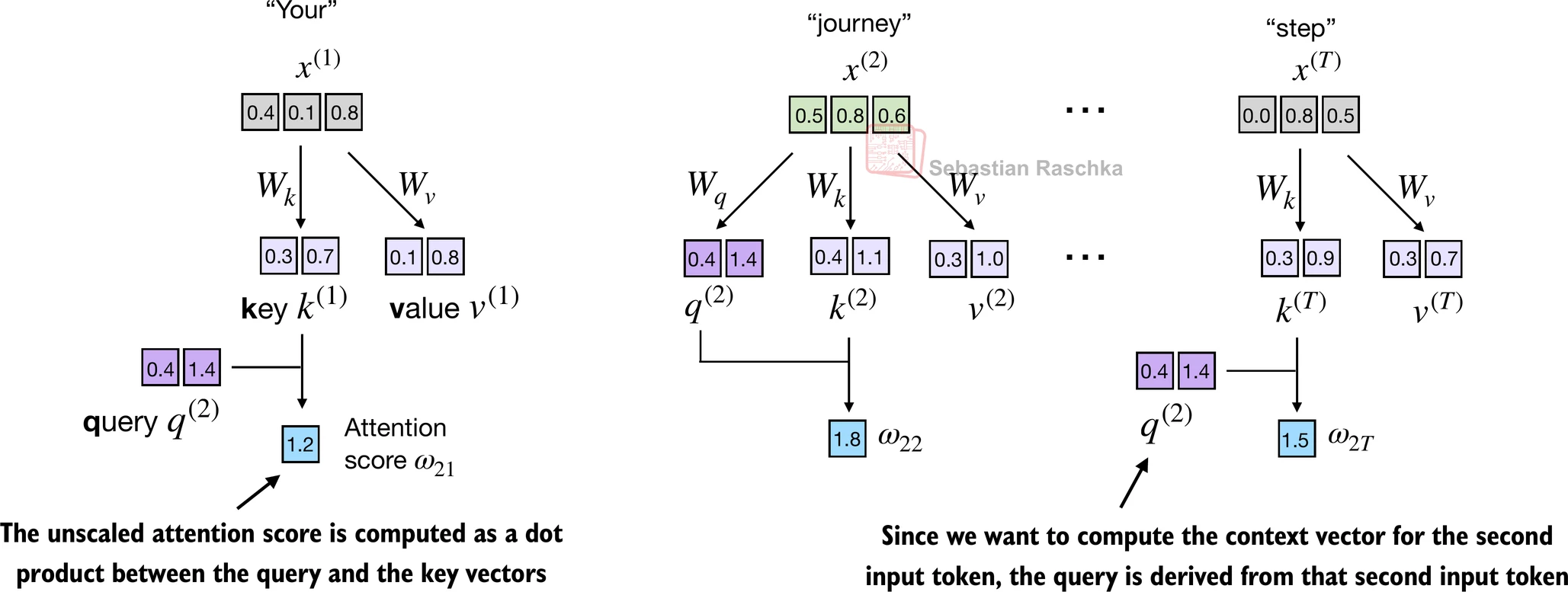
keys_2 = keys[1] # Python starts index at 0
attn_score_22 = query_2.dot(keys_2)
print(attn_score_22)
tensor(1.8524)
Since we have 6 inputs, we have 6 attention scores for the given query vector.
attn_scores_2 = query_2 @ keys.T # All attention scores for given query
print(attn_scores_2)
tensor([1.2705, 1.8524, 1.8111, 1.0795, 0.5577, 1.5440])
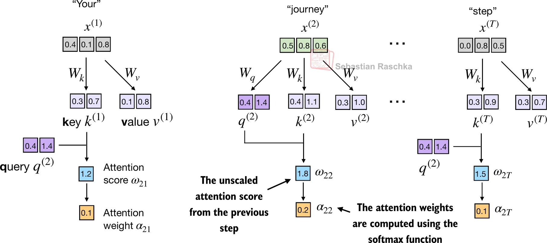
Step 3, we compute the attention weights (normalized attention scores that sum up to 1) using the softmax function we used earlier.
The difference to earlier is that we now scale the attention scores by dividing them by the square root of the embedding dimension, \sqrt{d_k} (i.e.,
d_k**0.5).The reason for the normalization by the embedding dimension size is to improve the training performance by avoiding small gradients that lead to gradient vanishing.
d_k = keys.shape[1]
attn_weights_2 = torch.softmax(attn_scores_2 / d_k**0.5, dim=-1)
print(attn_weights_2)
tensor([0.1500, 0.2264, 0.2199, 0.1311, 0.0906, 0.1820])
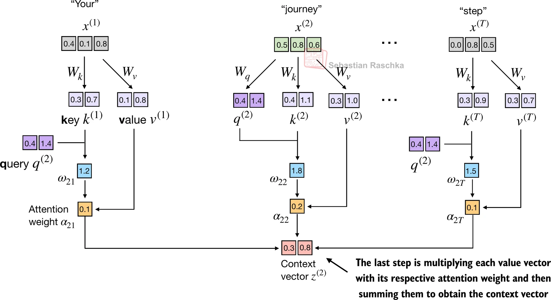
Step 4, we now compute the context vector for input query vector 2.
context_vec_2 = attn_weights_2 @ values
print(context_vec_2)
tensor([0.3061, 0.8210])
Putting all in SelfAttention class
Putting it all together, we can implement the self-attention mechanism as follows:
import torch.nn as nn

class SelfAttention_v1(nn.Module):

    def __init__(self, d_in, d_out):
        super().__init__()
        self.W_query = nn.Parameter(torch.rand(d_in, d_out))
        self.W_key   = nn.Parameter(torch.rand(d_in, d_out))
        self.W_value = nn.Parameter(torch.rand(d_in, d_out))

    def forward(self, x):
        keys = x @ self.W_key
        queries = x @ self.W_query
        values = x @ self.W_value

        attn_scores = queries @ keys.T # omega
        attn_weights = torch.softmax( # alpha (normalized omega)
            attn_scores / keys.shape[-1]**0.5, dim=-1
        )

        context_vec = attn_weights @ values
        return context_vec

torch.manual_seed(123)
sa_v1 = SelfAttention_v1(d_in, d_out)
print(sa_v1(inputs))
tensor([[0.2996, 0.8053],
[0.3061, 0.8210],
[0.3058, 0.8203],
[0.2948, 0.7939],
[0.2927, 0.7891],
[0.2990, 0.8040]], grad_fn=<MmBackward0>)
We can streamline the implementation above using PyTorch’s Linear layers, which are equivalent to a matrix multiplication if we disable the bias units.
Another big advantage of using nn.Linear over our manual nn.Parameter(torch.rand(...) approach is that nn.Linear has a preferred weight initialization scheme, which leads to more stable model training.
class SelfAttention_v2(nn.Module):

    def __init__(self, d_in, d_out, qkv_bias=False):
        super().__init__()
        self.W_query = nn.Linear(d_in, d_out, bias=qkv_bias)
        self.W_key   = nn.Linear(d_in, d_out, bias=qkv_bias)
        self.W_value = nn.Linear(d_in, d_out, bias=qkv_bias)

    def forward(self, x):
        keys = self.W_key(x)
        queries = self.W_query(x)
        values = self.W_value(x)

        attn_scores = queries @ keys.T
        attn_weights = torch.softmax(attn_scores / keys.shape[-1]**0.5, dim=-1)

        context_vec = attn_weights @ values
        return context_vec

torch.manual_seed(789)
sa_v2 = SelfAttention_v2(d_in, d_out)
print(sa_v2(inputs))
tensor([[-0.0739, 0.0713],
[-0.0748, 0.0703],
[-0.0749, 0.0702],
[-0.0760, 0.0685],
[-0.0763, 0.0679],
[-0.0754, 0.0693]], grad_fn=<MmBackward0>)
Hiding future words with causal attention
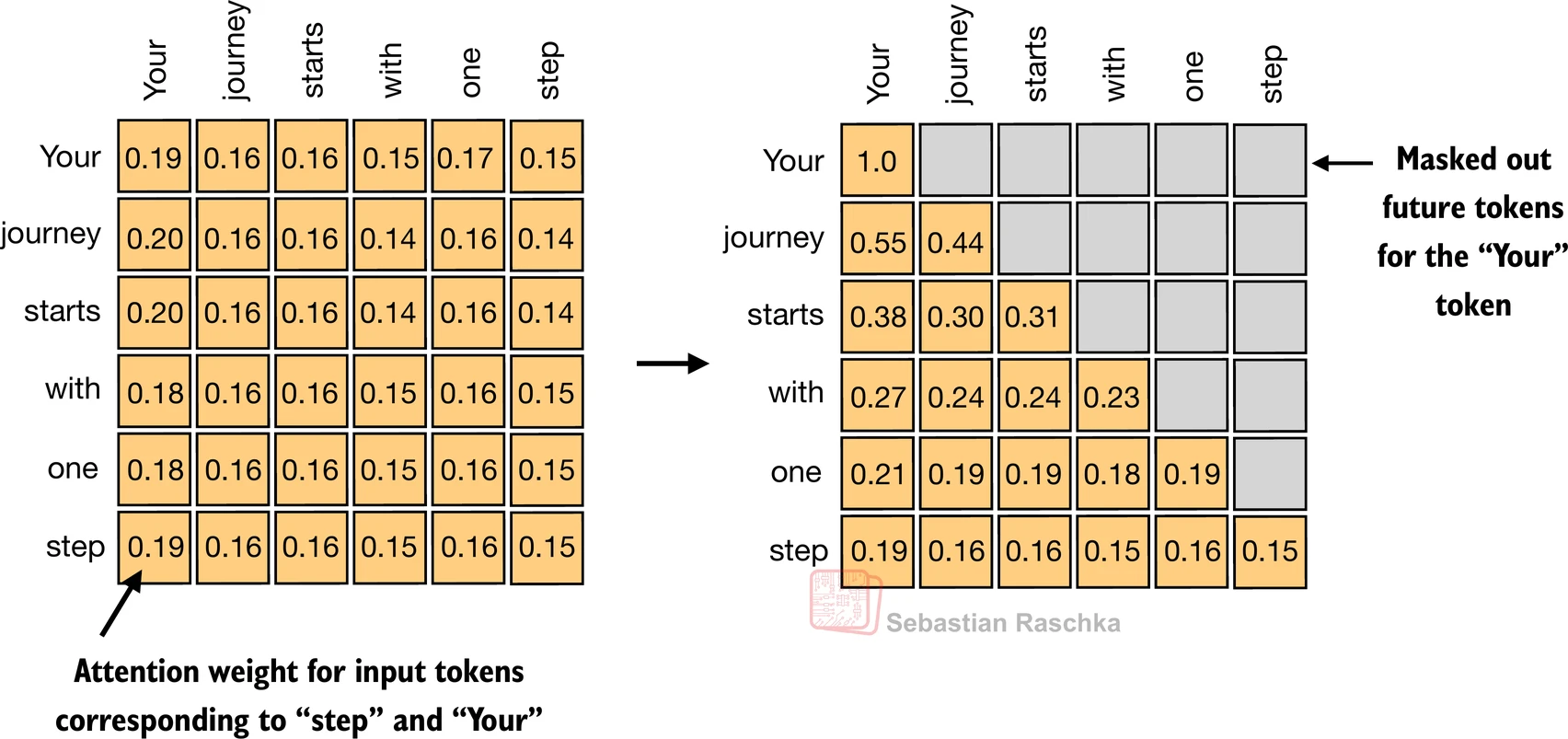
In causal attention, the attention weights above the diagonal are masked, ensuring that for any given input, the LLM is unable to utilize future tokens while calculating the context vectors with the attention weight.
Causal attention mask
Causal self-attention ensures that the model’s prediction for a certain position in a sequence is only dependent on the known outputs at previous positions, not on future positions.
To illustrate and implement causal self-attention, let’s work with the attention scores and weights from the previous section:
# Reuse the query and key weight matrices of the
# SelfAttention_v2 object from the previous section for convenience
queries = sa_v2.W_query(inputs)
keys = sa_v2.W_key(inputs)
attn_scores = queries @ keys.T

attn_weights = torch.softmax(attn_scores / keys.shape[-1]**0.5, dim=-1)
print(attn_weights)
tensor([[0.1921, 0.1646, 0.1652, 0.1550, 0.1721, 0.1510],
[0.2041, 0.1659, 0.1662, 0.1496, 0.1665, 0.1477],
[0.2036, 0.1659, 0.1662, 0.1498, 0.1664, 0.1480],
[0.1869, 0.1667, 0.1668, 0.1571, 0.1661, 0.1564],
[0.1830, 0.1669, 0.1670, 0.1588, 0.1658, 0.1585],
[0.1935, 0.1663, 0.1666, 0.1542, 0.1666, 0.1529]],
grad_fn=<SoftmaxBackward0>)
Create a mask via PyTorch’s tril function is the simplest way.
context_length = attn_scores.shape[0]
mask_simple = torch.tril(torch.ones(context_length, context_length))
print(mask_simple)
tensor([[1., 0., 0., 0., 0., 0.],
[1., 1., 0., 0., 0., 0.],
[1., 1., 1., 0., 0., 0.],
[1., 1., 1., 1., 0., 0.],
[1., 1., 1., 1., 1., 0.],
[1., 1., 1., 1., 1., 1.]])
Then, we can multiply the attention weights with this mask to zero out the attention scores above the diagonal.
masked_simple = attn_weights*mask_simple
print(masked_simple)
tensor([[0.1921, 0.0000, 0.0000, 0.0000, 0.0000, 0.0000],
[0.2041, 0.1659, 0.0000, 0.0000, 0.0000, 0.0000],
[0.2036, 0.1659, 0.1662, 0.0000, 0.0000, 0.0000],
[0.1869, 0.1667, 0.1668, 0.1571, 0.0000, 0.0000],
[0.1830, 0.1669, 0.1670, 0.1588, 0.1658, 0.0000],
[0.1935, 0.1663, 0.1666, 0.1542, 0.1666, 0.1529]],
grad_fn=<MulBackward0>)
However, if the mask were applied after softmax, like above, it would disrupt the probability distribution created by softmax. (Softmax ensures that all output values sum to 1)
In simpler terms, after masking and renormalization, the distribution of attention weights is as if it was calculated only among the unmasked positions to begin with. This ensures there’s no information leakage from future (or otherwise masked) tokens as we intended.
To make sure that the rows sum to 1 (prevent information leak), we can normalize the attention weights as follows:
row_sums = masked_simple.sum(dim=-1, keepdim=True)
masked_simple_norm = masked_simple / row_sums
print(masked_simple_norm)
tensor([[1.0000, 0.0000, 0.0000, 0.0000, 0.0000, 0.0000],
[0.5517, 0.4483, 0.0000, 0.0000, 0.0000, 0.0000],
[0.3800, 0.3097, 0.3103, 0.0000, 0.0000, 0.0000],
[0.2758, 0.2460, 0.2462, 0.2319, 0.0000, 0.0000],
[0.2175, 0.1983, 0.1984, 0.1888, 0.1971, 0.0000],
[0.1935, 0.1663, 0.1666, 0.1542, 0.1666, 0.1529]],
grad_fn=<DivBackward0>)
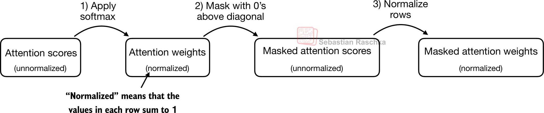
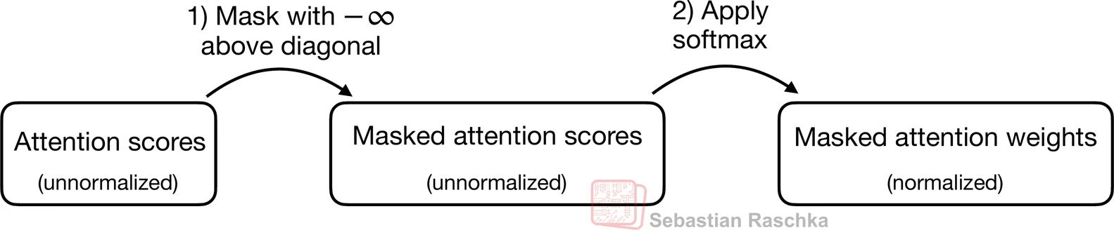
Be more efficent, instead of zeroing out attention weights above the diagonal and renormalizing the results, we can mask the unnormalized attention scores above the diagonal with negative infinity before they enter the softmax function:.
Softmax function treats as 0 during calculation.
mask = torch.triu(torch.ones(context_length, context_length), diagonal=1)
masked = attn_scores.masked_fill(mask.bool(), -torch.inf)
print(masked)
tensor([[0.2899, -inf, -inf, -inf, -inf, -inf],
[0.4656, 0.1723, -inf, -inf, -inf, -inf],
[0.4594, 0.1703, 0.1731, -inf, -inf, -inf],
[0.2642, 0.1024, 0.1036, 0.0186, -inf, -inf],
[0.2183, 0.0874, 0.0882, 0.0177, 0.0786, -inf],
[0.3408, 0.1270, 0.1290, 0.0198, 0.1290, 0.0078]],
grad_fn=<MaskedFillBackward0>)
As we can see below, now the attention weights in each row correctly sum to 1 again:
attn_weights = torch.softmax(masked / keys.shape[-1]**0.5, dim=-1)
print(attn_weights)
tensor([[1.0000, 0.0000, 0.0000, 0.0000, 0.0000, 0.0000],
[0.5517, 0.4483, 0.0000, 0.0000, 0.0000, 0.0000],
[0.3800, 0.3097, 0.3103, 0.0000, 0.0000, 0.0000],
[0.2758, 0.2460, 0.2462, 0.2319, 0.0000, 0.0000],
[0.2175, 0.1983, 0.1984, 0.1888, 0.1971, 0.0000],
[0.1935, 0.1663, 0.1666, 0.1542, 0.1666, 0.1529]],
grad_fn=<SoftmaxBackward0>)
Masking weights with dropout
In addition, we also apply dropout to reduce overfitting during training.
Dropout can be applied in several places:
for example, after computing the attention weights (more common);
or after multiplying the attention weights with the value vectors.
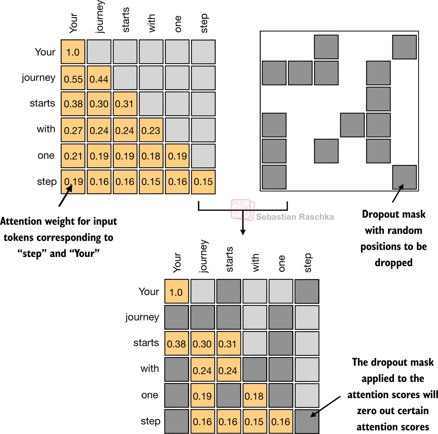
If we apply a dropout rate of 0.5 (50%), the non-dropped values will be scaled accordingly by a factor of 1/0.5 = 2.
The scaling is calculated by the formula 1 / (1 -
dropout_rate).
torch.manual_seed(123)
dropout = torch.nn.Dropout(0.5) # dropout rate of 50%
example = torch.ones(6, 6) # create a matrix of ones

print(dropout(example))
tensor([[2., 2., 0., 2., 2., 0.],
[0., 0., 0., 2., 0., 2.],
[2., 2., 2., 2., 0., 2.],
[0., 2., 2., 0., 0., 2.],
[0., 2., 0., 2., 0., 2.],
[0., 2., 2., 2., 2., 0.]])
torch.manual_seed(123)
print(dropout(attn_weights))
tensor([[0.3843, 0.3293, 0.0000, 0.3100, 0.3442, 0.0000],
[0.0000, 0.0000, 0.0000, 0.2992, 0.0000, 0.2955],
[0.4071, 0.3318, 0.3325, 0.2996, 0.0000, 0.2961],
[0.0000, 0.3334, 0.3337, 0.0000, 0.0000, 0.3128],
[0.0000, 0.3337, 0.0000, 0.3177, 0.0000, 0.3169],
[0.0000, 0.3327, 0.3331, 0.3084, 0.3331, 0.0000]],
grad_fn=<MulBackward0>)
Compact causal self-attention class
One more thing is to implement the code to handle batches consisting of more than one input so that our CausalAttention class supports the batch outputs produced by the data loader.
batch = torch.stack((inputs, inputs), dim=0)
print(batch.shape) # 2 inputs with 6 tokens each, and each token has embedding dimension 3
torch.Size([2, 6, 3])
class CausalAttention(nn.Module):

    def __init__(self, d_in, d_out, context_length,
                 dropout, qkv_bias=False):
        super().__init__()
        self.d_out = d_out
        self.W_query = nn.Linear(d_in, d_out, bias=qkv_bias)
        self.W_key   = nn.Linear(d_in, d_out, bias=qkv_bias)
        self.W_value = nn.Linear(d_in, d_out, bias=qkv_bias)
        self.dropout = nn.Dropout(dropout) # New
        self.register_buffer('mask', torch.triu(torch.ones(context_length, context_length), diagonal=1)) # New

    def forward(self, x):
        b, num_tokens, d_in = x.shape # New batch dimension b
        # For inputs where `num_tokens` exceeds `context_length`, this will result in errors
        # in the mask creation further below.
        # In practice, this is not a problem since the LLM (chapters 4-7) ensures that inputs
        # do not exceed `context_length` before reaching this forward method.
        keys = self.W_key(x)
        queries = self.W_query(x)
        values = self.W_value(x)

        attn_scores = queries @ keys.transpose(1, 2) # Changed transpose
        attn_scores.masked_fill_(  # New, _ ops are in-place
            self.mask.bool()[:num_tokens, :num_tokens], -torch.inf)  # `:num_tokens` to account for cases where the number of tokens in the batch is smaller than the supported context_size
        attn_weights = torch.softmax(
            attn_scores / keys.shape[-1]**0.5, dim=-1
        )
        attn_weights = self.dropout(attn_weights) # New

        context_vec = attn_weights @ values
        return context_vec

torch.manual_seed(123)

context_length = batch.shape[1]
ca = CausalAttention(d_in, d_out, context_length, 0.0)

context_vecs = ca(batch)

print(context_vecs)
print("context_vecs.shape:", context_vecs.shape)
tensor([[[-0.4519, 0.2216],
[-0.5874, 0.0058],
[-0.6300, -0.0632],
[-0.5675, -0.0843],
[-0.5526, -0.0981],
[-0.5299, -0.1081]],
[[-0.4519, 0.2216],
[-0.5874, 0.0058],
[-0.6300, -0.0632],
[-0.5675, -0.0843],
[-0.5526, -0.0981],
[-0.5299, -0.1081]]], grad_fn=<UnsafeViewBackward0>)
context_vecs.shape: torch.Size([2, 6, 2])
Note that dropout is only applied during training, not during inference
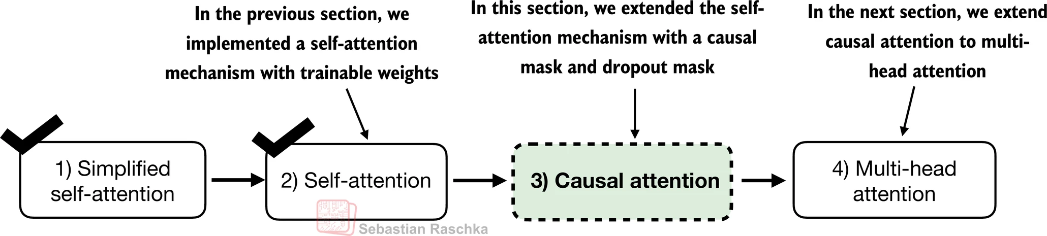
Multi-head attention
Stacking single-head attention
Single-head attention (What we just went through.)
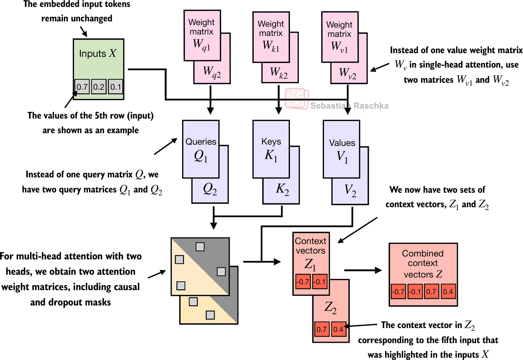
Multi-head attention: Stack multiple single-head attention.
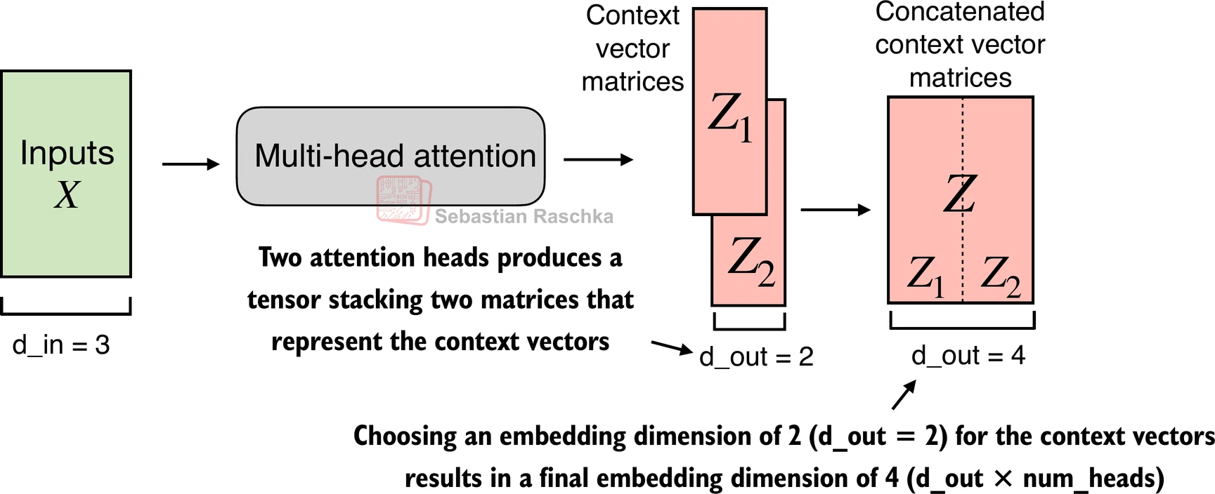
The main idea is to run the attention mechanism multiple times (in parallel) with different, learned linear projections. This allows the model to jointly attend to information from different representation subspaces at different positions.
The following code uses the previous CausalAttention class for illustration. (In the next section will reveal more.)
class MultiHeadAttentionWrapper(nn.Module):

    def __init__(self, d_in, d_out, context_length, dropout, num_heads, qkv_bias=False):
        super().__init__()
        self.heads = nn.ModuleList(
            [CausalAttention(d_in, d_out, context_length, dropout, qkv_bias)
             for _ in range(num_heads)]
        )

    def forward(self, x):
        return torch.cat([head(x) for head in self.heads], dim=-1)


torch.manual_seed(123)

context_length = batch.shape[1] # This is the number of tokens
d_in, d_out = 3, 2
mha = MultiHeadAttentionWrapper(
    d_in, d_out, context_length, dropout=0.0, num_heads=2
)

context_vecs = mha(batch)

print(context_vecs)
print("context_vecs.shape:", context_vecs.shape) # dimension changes
tensor([[[-0.4519, 0.2216, 0.4772, 0.1063],
[-0.5874, 0.0058, 0.5891, 0.3257],
[-0.6300, -0.0632, 0.6202, 0.3860],
[-0.5675, -0.0843, 0.5478, 0.3589],
[-0.5526, -0.0981, 0.5321, 0.3428],
[-0.5299, -0.1081, 0.5077, 0.3493]],
[[-0.4519, 0.2216, 0.4772, 0.1063],
[-0.5874, 0.0058, 0.5891, 0.3257],
[-0.6300, -0.0632, 0.6202, 0.3860],
[-0.5675, -0.0843, 0.5478, 0.3589],
[-0.5526, -0.0981, 0.5321, 0.3428],
[-0.5299, -0.1081, 0.5077, 0.3493]]], grad_fn=<CatBackward0>)
context_vecs.shape: torch.Size([2, 6, 4])
In the implementation above, the embedding dimension is 4, because we d_out=2 as the embedding dimension for the key, query, and value vectors as well as the context vector. And since we have 2 attention heads, we have the output embedding dimension 2*2=4.
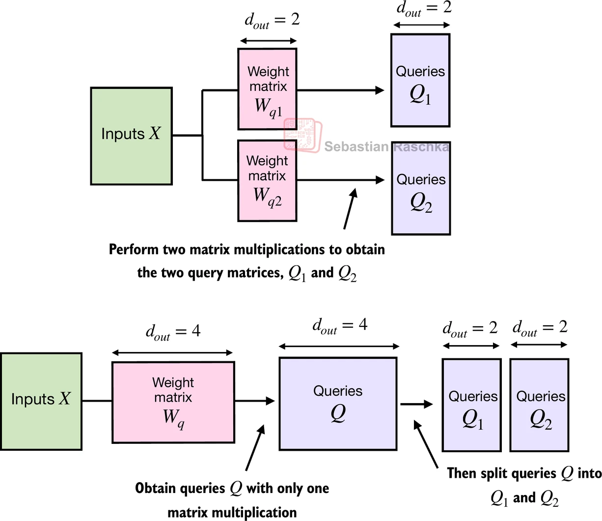
More efficient with weight splits
Now, we don’t concatenate single attention heads for this stand-alone MultiHeadAttention class. Instead, we create single W_query, W_key, and W_value weight matrices and then split those into individual matrices for each attention head:
class MultiHeadAttention(nn.Module):
    def __init__(self, d_in, d_out, context_length, dropout, num_heads, qkv_bias=False):
        super().__init__()
        assert (d_out % num_heads == 0), \
            "d_out must be divisible by num_heads"

        self.d_out = d_out
        self.num_heads = num_heads
        self.head_dim = d_out // num_heads # Reduce the projection dim to match desired output dim

        self.W_query = nn.Linear(d_in, d_out, bias=qkv_bias)
        self.W_key = nn.Linear(d_in, d_out, bias=qkv_bias)
        self.W_value = nn.Linear(d_in, d_out, bias=qkv_bias)
        self.out_proj = nn.Linear(d_out, d_out)  # Linear layer to combine head outputs
        self.dropout = nn.Dropout(dropout)
        self.register_buffer(
            "mask",
            torch.triu(torch.ones(context_length, context_length),
                       diagonal=1)
        )

    def forward(self, x):
        b, num_tokens, d_in = x.shape
        # As in `CausalAttention`, for inputs where `num_tokens` exceeds `context_length`,
        # this will result in errors in the mask creation further below.
        # In practice, this is not a problem since the LLM (chapters 4-7) ensures that inputs
        # do not exceed `context_length` before reaching this forward method.

        keys = self.W_key(x) # Shape: (b, num_tokens, d_out)
        queries = self.W_query(x)
        values = self.W_value(x)

        # We implicitly split the matrix by adding a `num_heads` dimension
        # Unroll last dim: (b, num_tokens, d_out) -> (b, num_tokens, num_heads, head_dim)
        keys = keys.view(b, num_tokens, self.num_heads, self.head_dim)
        values = values.view(b, num_tokens, self.num_heads, self.head_dim)
        queries = queries.view(b, num_tokens, self.num_heads, self.head_dim)

        # Transpose: (b, num_tokens, num_heads, head_dim) -> (b, num_heads, num_tokens, head_dim)
        keys = keys.transpose(1, 2)
        queries = queries.transpose(1, 2)
        values = values.transpose(1, 2)

        # Compute scaled dot-product attention (aka self-attention) with a causal mask
        attn_scores = queries @ keys.transpose(2, 3)  # Dot product for each head

        # Original mask truncated to the number of tokens and converted to boolean
        mask_bool = self.mask.bool()[:num_tokens, :num_tokens]

        # Use the mask to fill attention scores
        attn_scores.masked_fill_(mask_bool, -torch.inf)

        attn_weights = torch.softmax(attn_scores / keys.shape[-1]**0.5, dim=-1)
        attn_weights = self.dropout(attn_weights)

        # Shape: (b, num_tokens, num_heads, head_dim)
        context_vec = (attn_weights @ values).transpose(1, 2)

        # Combine heads, where self.d_out = self.num_heads * self.head_dim
        context_vec = context_vec.contiguous().view(b, num_tokens, self.d_out)
        context_vec = self.out_proj(context_vec) # optional projection

        return context_vec

torch.manual_seed(123)

batch_size, context_length, d_in = batch.shape
d_out = 2
mha = MultiHeadAttention(d_in, d_out, context_length, 0.0, num_heads=2)

context_vecs = mha(batch)

print(context_vecs)
print("context_vecs.shape:", context_vecs.shape)
tensor([[[0.3190, 0.4858],
[0.2943, 0.3897],
[0.2856, 0.3593],
[0.2693, 0.3873],
[0.2639, 0.3928],
[0.2575, 0.4028]],
[[0.3190, 0.4858],
[0.2943, 0.3897],
[0.2856, 0.3593],
[0.2693, 0.3873],
[0.2639, 0.3928],
[0.2575, 0.4028]]], grad_fn=<ViewBackward0>)
context_vecs.shape: torch.Size([2, 6, 2])
Note that in addition, we added a linear projection layer (self.out_proj ) to the MultiHeadAttention class above. This is simply a linear transformation that doesn’t change the dimensions. It’s a standard convention to use such a projection layer in LLM implementation, but it’s not strictly necessary. (Recent research has shown that it can be removed without affecting the modeling performance.)
Check out
torch.nn.MultiheadAttentionclass in PyTorch.
Since the above implementation may look a bit complex at first glance, let’s look at what happens when executing attn_scores = queries @ keys.transpose(2, 3):
# (b, num_heads, num_tokens, head_dim) = (1, 2, 3, 4)
a = torch.tensor([[[[0.2745, 0.6584, 0.2775, 0.8573],
                    [0.8993, 0.0390, 0.9268, 0.7388],
                    [0.7179, 0.7058, 0.9156, 0.4340]],

                   [[0.0772, 0.3565, 0.1479, 0.5331],
                    [0.4066, 0.2318, 0.4545, 0.9737],
                    [0.4606, 0.5159, 0.4220, 0.5786]]]])

print(a @ a.transpose(2, 3))
tensor([[[[1.3208, 1.1631, 1.2879],
[1.1631, 2.2150, 1.8424],
[1.2879, 1.8424, 2.0402]],
[[0.4391, 0.7003, 0.5903],
[0.7003, 1.3737, 1.0620],
[0.5903, 1.0620, 0.9912]]]])
In this case, the matrix multiplication implementation in PyTorch will handle the 4-dimensional input tensor so that the matrix multiplication is carried out between the 2 last dimensions (num_tokens, head_dim) and then repeated for the individual heads.
For instance, the following becomes a more compact way to compute the matrix multiplication for each head separately:
first_head = a[0, 0, :, :]
first_res = first_head @ first_head.T
print("First head:\n", first_res)

second_head = a[0, 1, :, :]
second_res = second_head @ second_head.T
print("\nSecond head:\n", second_res)
First head:
tensor([[1.3208, 1.1631, 1.2879],
[1.1631, 2.2150, 1.8424],
[1.2879, 1.8424, 2.0402]])
Second head:
tensor([[0.4391, 0.7003, 0.5903],
[0.7003, 1.3737, 1.0620],
[0.5903, 1.0620, 0.9912]])
Prepare for interview
Code from scratch:
SelfAttention_v2,CausalAttention,MultiHeadAttention.